Geometry of Distributed Representations

September 17, 2024 • David Bau

Today we begin a segment of the class dealing with understanding representations: understanding the ways that information might be encoded in the patterns of neural activations in a neural network.

In the previous chapter on neurons, we examined some of the efforts to visualize and understand the "concepts" that might be represented by individual neurons in an artificial neural network. The idea that individual neurons might directly correspond to interpretable variables is the "Local Representation" hypothesis. As we saw, some individual neurons do seem encode specific concepts. However, in practice, many other individual neurons seem to lack clear mappings to discrete understandable concepts.

Hinton, McClelland, and Rumelhart have advocated the view that all the neurons work together to store the aggregate information in a network, and further that that this collective cooperation is essentially irreducible. The hypothesis that every neuron is involved in encoding many different concepts is the Distributed Representation model, and they have advocated this viewpoint since their 1987 work "Parallel Distributed Processing" (PDP). This distributed representation view is the prevailing view among neuoscientists; (most believe that the local view of individual neurons as concepts is not true).

If information is inherently distributed, then instead of examining individual neurons $ h_i \in \mathbb{R} $ as scalar variables, we should examine the vector space $ \mathbf{h} \in \mathbb{R}^N $ of all the neurons together; we call this collective vector space the representation space of the network. In a feedforward neural network, each layer of neurons is a bottleneck that fully determines all the subsequent information in a network, so we will typically look at the representation vector for the neurons in a single layer $ \mathbf{h} \in \mathbb{R}^d $, where the dimensionality $ d $ is given by the number of neurons in a layer.

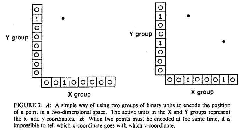
In 1987, the PDP authors examined several possible ways of encoding information in a distributed fashion within a representation vector space. For example, in their Figure 2 (pictured above), they observed the following dilemma. Suppose neurons collaborate in two groups to encode an $ (x, y) $ combination, like a point on a plane. It leads to the problem that if you use the same scheme to encode two points, there is not an ambiguity for which $ x $ goes with which $ y $. Thus they faced a puzzle: when sets of neurons distribute information, how do they encode it effectively?

The Meaning of Right Angles

We begin today by looking at two recent papers that tackle this representation encoding question from a geometric point of view. Both begin can be seen as a contemplation of the question:

Why don't vectors for independent features lie at right angles in representation space?

Notice that each individual neuron defines a simple representation vector $e_i$ that has a 1 in the $i$th spot and 0 in all the other spots, so if each neuron were an independent feature, then they would all lie at right angles since $e_i \cdot e_j = 0$ for all $i \neq j$. But both papers notice that, in practice, vectors for features do not seem to correspond to individual neurons, and moreover, vectors $v_i$ that seem to represent independent features do not even satisfy $v_i \cdot v_j = 0$ in general. Both papers ask: why not?

The two papers motivate this question from very different starting points. Then they arrive at two very different answers to this question.

Toy Models of Superposition

The paper Toy Models of Superposition is a blog post by Nelson Elhage and Chris Olah's group at Anthropic in collaboration with Martin Wattenberg at Harvard. (As an aside: you might wonder why this was published as a blog instead of a pdf paper. For years, Olah has been a big advocate of publishing research in non-traditionally-peer-reviewed blog formats.)

The Goal: Enumeration

To understand the motivation of the paper, it is helpful to start at the end; in their section 9, they explain that they would like to understand how to enumerate all the features in a representation:

We'd like a way to have confidence that models will never do certain behaviors such as "deliberately deceive" or "manipulate." Today, it's unclear how one might show this, but we believe a promising tool would be the ability to identify and enumerate over all features.

This team had previously developed catalogs of neurons (as we read about) when they previously worked at OpenAI. They note that if each interpertable variable corresponded to one neuron, then "you could enumerate over features by enumerating over neurons." Yet if we are in a distributed representation where every neuron is involved in encoding multple variables, then it leaves you with an unsolved problem: if the way each variable is encoded is unknown, it becomes unclear how to find the representations of all the variables, or even how to identify what the variables are.

Nevertheless, the Elhage team is optimistic that it should be possible to enumerate the variables, if we can somehow reverse-engineer the distributed representation encodings learned by a neural network.

The Data: Synthetic Sparse Features

To begin to tackle this reverse-engineering problem, the paper takes the approach of training very small neural networks on very small problems for which they can define a ground truth for the "interpretable variables." Then they ask: what is the actual learned encoding? How does the network represent information about these variables?

To play the role of interpretable variables, they propose "sparse features." A sparse feature is a variable that is typically zero, but that becomes positive in the rare but interesting situations where there is something to say. (Hinton 1987 wrote about this idea; Elhage also suggests reading Olshausen 1997.) For example, a sparse feature might be the information "there is a dog's head in the photo." Since most photos don't include dog heads, it's usually zero, but sometimes it is positive, and it could be a large number if there are lot of dogs in a specific instance (for example).

In their various experiments, Elhage does not use "real" data for features but rather synthesizes random sparse features, which gives them control over the following two characteristics for each feature $ x_i $:

$ S_i $ is the sparsity of the $i$th feature, that is the probabilitity it is zero.

$ I_i $ is the importance of the $i$th feature, the cost incurred if information about it was lost.

For example, if $ (1 - S_i) = 0.01 $, then the $ i $th feature is nonzero only 1\% of the time.

And if $ I_i = 2 $ and $ I_j = 1 $, then the $ i $th feature has twice the weight of the $ j $th feature in the reconstruction loss.

For most of their experimens, they choose a uniform sparsity $ S $ for all the features and select a varying importance and $ I_i $ for each of $ n $ features, and then they synthesize fake data by creating random vectors $ [ x_1, x_2, ..., x_n ] $ that follow the sparsity probabilities. They use this data to train neural networks on various tasks, then analyze the representations that are learned. Since they know the exact values and characteristics of their sparse features, they can measure how those characteristics relate to different types of representations.

The Tasks: Autoencoding, Adversarial Attack, and Absolute Value

The basic task they examine is autoencoding: learning a two-layer network that can squeeze the information of many features $ x_i $ through a smaller number of hidden unit neurons, while still being able to reconstruct $ x_i $ in the end.

They make two unusual choices. One is to begin by studying a totally linear network with no nonlinearities in the middle. The other is to constrain the second network layer to have the same weights as the first, just transposed. That is, the first layer has weights that act as follows: \[ h = Wx = \left[ \begin{array}{c|c|c|c} \phantom{0} & \phantom{0} & & \phantom{0} \\ w_1 & w_2 & ... & w_n \\ \phantom{0} & \phantom{0} & & \phantom{0} \end{array} \right] \begin{bmatrix} x_1 \\ x_2 \\ \vdots \\ x_n \end{bmatrix} = \sum_i w_i x_i \]

And then the second layer has exactly the same weights, but transposed: \[ \hat{x} = W^T h = \begin{bmatrix} \phantom{0} & w_1^T & \phantom{0} \\ \hline \phantom{0} & w_2^T & \phantom{0} \\ \hline & \vdots & \\ \hline \phantom{0} & w_n^T & \phantom{0} \end{bmatrix} h = \begin{bmatrix} w_1^T h \\ w_2^T h \\ \vdots \\ w_n^T h \end{bmatrix} \]

In other words: the first matrix is an embedding matrix that encodes the $i$th feature as the vector $w_i$, and the second matrix is a projection matrix that decodes the $i$th feature by using the (Euclidean) inner product that evaluates the component in the direction of $w_i$ again. For both encoding and decoding $w_i$ can be thought of as the vector embedding of the $i$th feature.

With this basic starting point, they train the following variations:

Fully linear autoencoding: $ \hat{x} = W^T W x + b$, with $ \hat{x}_i \rightarrow x_i $.

Rectified linear autoencoding: $ \hat{x} = \mathrm{ReLU}(W^T W x + b) $, with $ \hat{x}_i \rightarrow x_i $.

Adversarial attack: $ \hat{x} = \mathrm{ReLU}(W^T W (x + \epsilon + b) $, with $ \epsilon $ chosen to maximize error in $\hat{x}$.

Absolute value: $ \hat{x} = \mathrm{ReLU}(W_2^T \mathrm{ReLU}(W_1 x) + b) $, with $ \hat{x}_i \rightarrow |x_i| $.

(The "absolute value" setting is the most conventional neural network setting, discarding the coupling of the weights and introducing a nonlinearity at the hidden layer.)

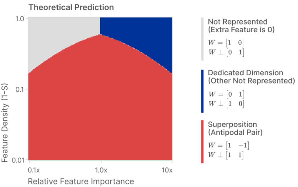
Conditions that Lead to Superposition

The main finding of the paper is the counterintuitive result that sparsity in the underlying features that is $ (1 - S) $ close to zero, leads to more superposition and more entanglement, rather than less.

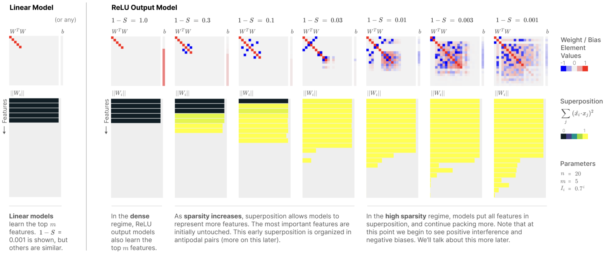
The ordinary boring solution for the network, shown on the left of the figure above is what they call "PCA-like behavior". When PCA is used to encode an $n$ dimiensional problem in a smaller $m$ dimensional space, PCA simply finds the most important vector directions in the distribution, directly encodes those, and then drops all the other directions, setting those components to zero. They found that without nonlinearities, training always resulted in this PCA choice. They also found that, even with nonlinearities, the PCA choice was found when the data was not sparse, i.e., when all the features were active most of the time.

However, when we have both sparsity and nonlinearity, then the network exploits an opportunity to encode more than $m$ features within the $m$-dimensional vector space. This sacrifices the orthogonal independence of the $w_i$ feature embedding vectors, as shown in this figure:

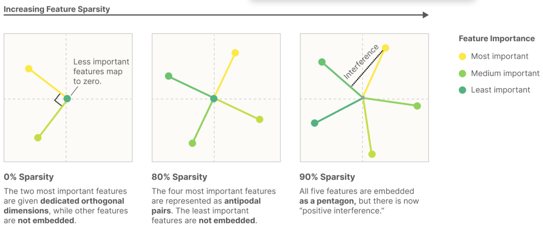
Thus, they argue, that the entanglement seen in distributed representations is inevitable: it's not just about a choice of basis that is unknown, but it is about a choice of embedding that overcrowds the available dimensions, and that does not cleanly correspond to a basis.

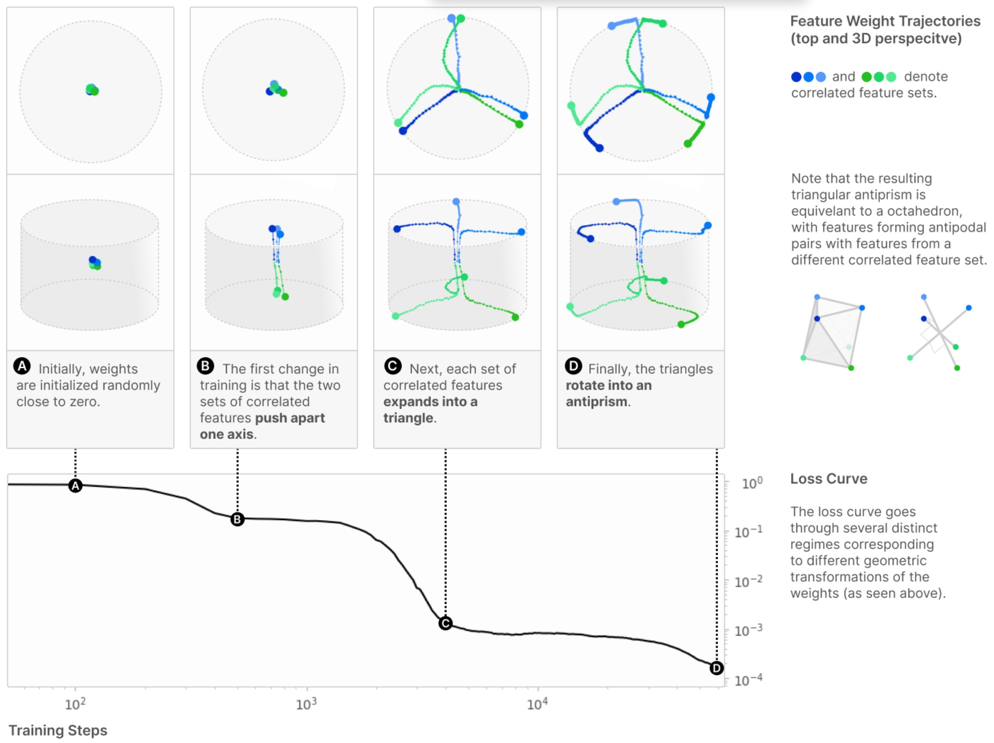
They supply a very nice python notebook that derives an exact solution for the optimal "amount" of dimensionality that should be allocated to each feature, and they show that this model matches what is found by the optimizer in practice.

Then they examine learning dynamics and the exact geometry of the layout of the vectors that are learned when they are in superposition, and they find some pretty symmetries that correspond to the optimizer finding the corners of regular polytopes in low dimensions.

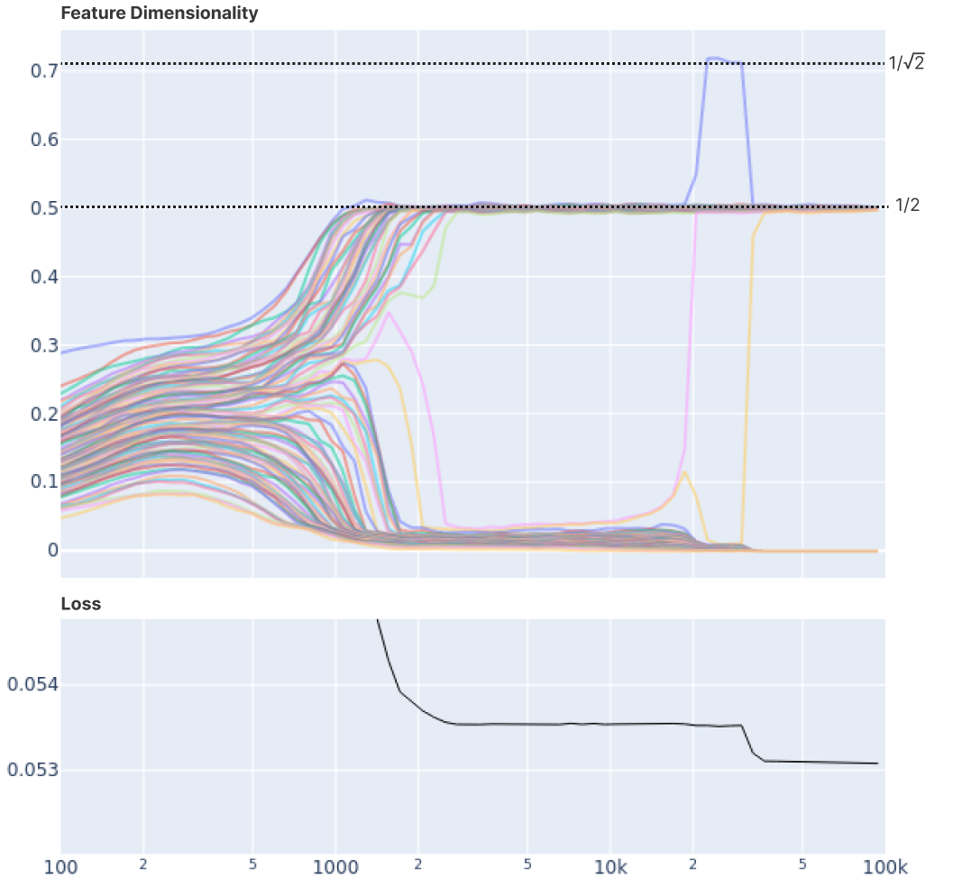
"Fractional Dimensions," Superposition, and Adversarial Attack

One of the interesting quantities defined by the paper is their fractional "dimension". In an ordinary PCA solution, all the feature vectors $ w_i $ are orthogonal and consume a whole dimension, leaving space for only $m$ features to be represented. But they observe that a feature in superposition with other features will consume less than a whole dimension, and they quantify the "dimensionality" of the $i$th feature as: \[ d_i = \frac{ ||w_i||^2 } { \sum_{j} (\hat{w}_i \cdot w_j)^2 } = \frac{ ||w_i||^4 }{\sum_{j} (w_{i} \cdot w_j)^2 } \]

Plotting this dimensionality measure over time reveals a satsifying discreteness to the solutions that correspond to the symmetric-geometry solutions, for example, where a feature goes to "1/2" a dimension when the dimension is shared with one other feature, and jumps higher as it starts consuming more space in the representation.

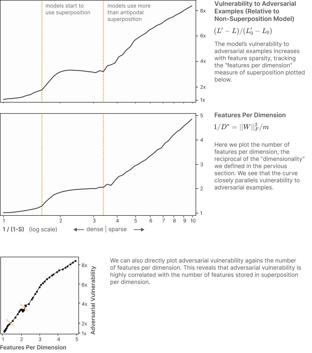
The paper also hypothesizes that the success of adversarial attacks hinges on this overpacking of features into dimensions, plotting a clear corrfelation between the (reciprocal of) the dimension measure and the vulnerability of the model to adversarial attack.

The Linear Representation Hypothesis

The Linear Representation Hypothesis paper by Park, Choe, and Veitch (ICML 2024) examines the geometry of representation spaces from a very different perspective: instead of focusing on a "dimension overloading" phenomenon in which underlying features are inherently entangled, they hypothesize that useful underlying features are disentangled and orthogonal to each other if you define orthogonality in the right way.

To define orthogonality, they introduce a concept they call the Causal Inner Product.

The rough idea is this: if you have representation vectors representing concepts $W$ and $Z$, then ideally, if the two concepts are indepenent, then their corresponding representation vectors should be orthogonal. However, this rough idea needs to be refined to make things work: Park defines concepts in a certain way, and then introduces causal separation instead of indepedence; then defines what a good unembedding vector would be an separately an embedding vector for a concept; then finally introduces the causal inner product instead of Euclidean geometry.

The Data: Semantic Vector Offset Directions

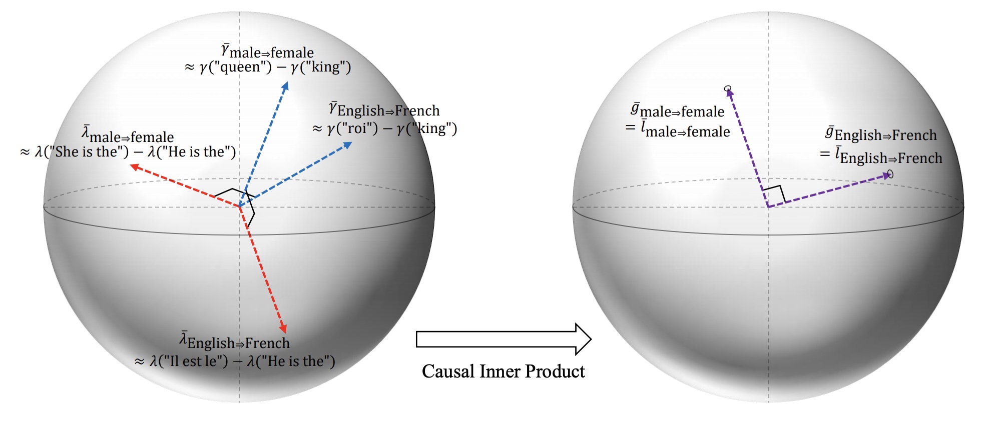
Concept variables as changes. First, Park assumes that a concept variable is a transformation of an attribute from one value to another, for example "male⇒female".

Unembedding vectors lead directly to an output change. Language models have two ways of looking at the embedding spaces: first, you can look at each vector as encoding a "next word to output". Park uses the symbol $\gamma$ to describe a vector that will cause a particular word to be output, and defines the "unembedding" vector for a concept as the vector difference $\gamma(Y(1)) - \gamma(Y(0)$, which is his notation for, for example, $\gamma(\text{“woman"}) - \gamma(\text{“man"})$ for the "man⇒woman" concept. If you look at the source code for the project, you can see that, in practice, these $\gamma$ vectors are just read directly (mean-centered) columns of the decoding matrix of a transformer.

Embedding vectors encode a narrowly specific input change. The second way to look at embedding vectors is that they are a response to input text. Park writes, e.g., $\lambda_0 = \lambda(\text{“He is the monarch of England,"})$, or $\lambda_1 = \lambda(\text{“She is the monarch of England,"})$, to describe these vectors, and proposes that a vector for a concept is similarly a vector difference $\lambda_1 - \lambda_0$ corresponding to the narrow concept change from one sentence to other. If you look at the source code for the project, it appears that, in practice these $\lambda$ vectors are read directly from the last-token last-layer hidden state of the transformer after processing some input text.

Causal separation. Park explains: causally separable concepts are those that can be varied freely and in isolation. For example, "English⇒French" and "male⇒female" are causally separable, whereas "English⇒Russian" is not separable from "English⇒French". This definition pulls a lot of weight in Park's proofs: for example, Park says that an vector for a concept is only a good embedding vector for a concept $W$ if adding the vector does not change the probability of any causally separated concetpts $Z$. I.e., he takes this as the definition for an embedding vector.

Defining a Causal Inner Product

Causal inner product. Then finally: Park wants vectors for concepts to be orthogonal if the concepts are causally separable. But he realizes this will not the case without an adjustment. Instead of using the ordinary inner product $ \gamma \cdot \gamma' $ to relate two vectors, he proposes a covariance-corrected inner product: \[ \langle \bar{\gamma}, \bar{\gamma}' \rangle_C = \bar{\gamma}^T \mathrm{Cov}(\gamma)^{-1} \bar{\gamma}' \]

In practice in the code, this covariance matrix is read directly from the decoding head of the model. Park argues (he writes some proofs, but I think there might be some gaps in his assumptions) that when the causal inner product is used instead of the regular inner product, then causally separable concepts will be orthogonal to each other, i.e., $ \langle \gamma_W, \gamma_Z \rangle = 0 $ for separable $W$ and $Z$.

Park notes that if you transform embedding space through the square-root of this covariance correction, e.g., if you define \[ \bar{g} = A\bar{\gamma} \quad \text{ where } \quad A = \mathrm{Cov}(\gamma)^{-1/2} \]

Then within the transformed vector space of $\bar{g}$, the ordinary Euclidean dot product acts like the causal inner product.

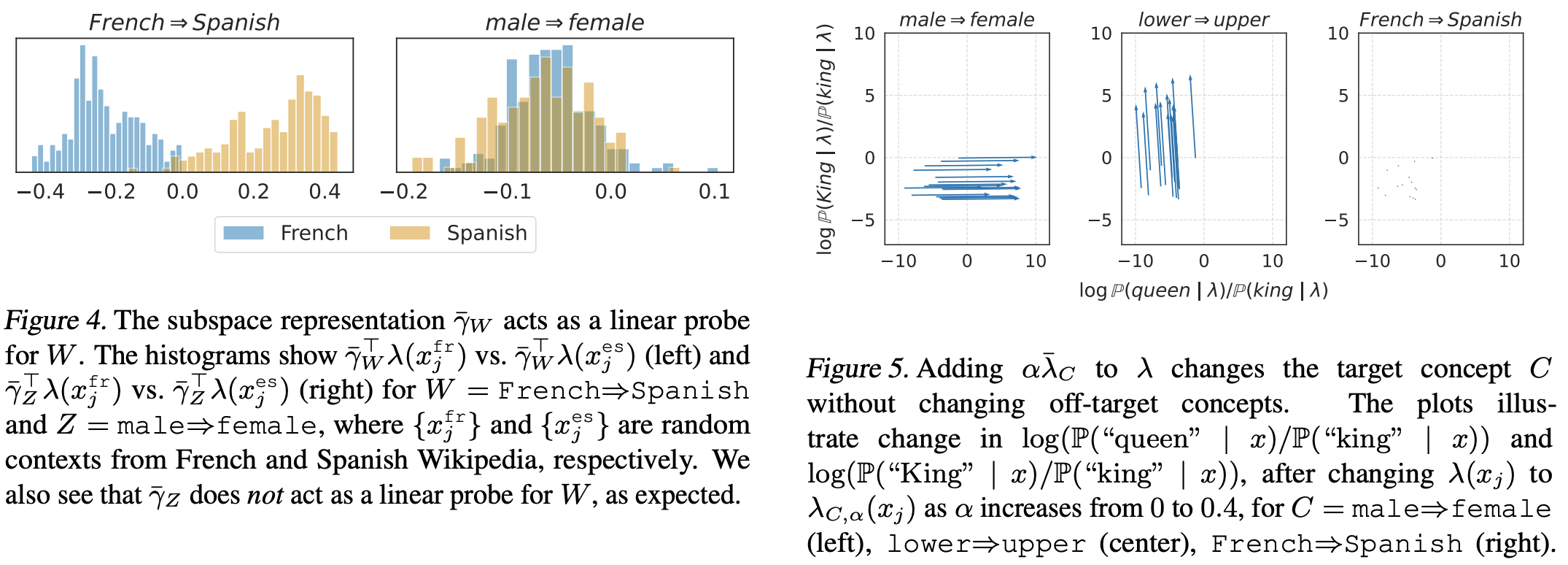
Experimental Checks

To check their hypothesized geometrical intutions, they use this covariance-corrected geometry to test several things - interestingly, even though the geometry is totally based on covariances in the output embeddings, they seem to achieve good separation when making target changes of a concept on inputs.

The paper builds upon a 2023 paper from the Veitch lab Concept Algebra by Wang, which does a similar thing in diffusion models.

(A research note - in our the Bau lab, we have several works that use a similar technique - Rewriting a generative model, the ROME paper and the Unified Concept Editing papers make similar covariance corrections in order to align geometric orthogonality with statistical indepdnence - but we do covariance corrections based on input statistics and Park corrects based on the output embedding matrix. It's reasonable to ask whether these are the same or different, and why.)

Code resources

The "Toy Models" paper comes with two notebooks: the link_text includes some efficient training code that can reproduce some of the larger experiments in the paper, but it is not very well-explained. A more valuable starting point is the link_text that explains several things that are glossed over in the main paper.

The "Linear Representation" paper comes with a github repo, and the most interesting code is in these files store_matrices.py and linear_rep_geometry.py.

Discussion Questions

Why are these research groups so interested in the geometry of vector spaces? What does vector space geometry have to do with interpretability of deep networks?
Think about the contrast between Elhage's focus on discerning latent sparse features, and Park's focus on geometry of inner products in the space. Do these viewpoints contradict each other? And think about the way the two papers were presented differently; which parts of their presentation and reasoning do you find convincing, or not, and why?